What is Q-Learning?

What are the Core Algorithmic Characteristics of Q-Learning?

Q-learning is defined by three primary algorithmic characteristics:

• Model-free: The algorithm does not require a complex transition model or any prior knowledge of environmental dynamics to function.
• Value-based: It operates by iteratively optimizing a discrete value function—the Q-function—to strictly dictate behavior.
• Off-policy: The behavior policy utilized to explore the environment during training differs entirely from the update policy being learned and mathematically optimized.

Historically, Q-learning was introduced by Watkins in 1989. Standard Q-learning provided the precise foundational mechanics that eventually led to modern deep reinforcement learning achievements, heavily influencing advancements such as AlphaGo and modern reinforcement learning from human feedback (RLHF) techniques.

What are the Building Blocks of Q-Learning?

A robust understanding of Q-learning requires defining the specific mathematical and conceptual entities that constitute a Markov decision process. These strict building blocks establish the rules of engagement between the learning algorithm and its operational environment.

The foundational mathematical framework underlying Q-learning is known as the Markov Decision Process (MDP). An MDP is formally defined as a tuple consisting of defined states, permissible actions, transition probabilities, environmental rewards, and a mathematical discount factor. This framework relies on the Markov property, asserting that the future state depends strictly upon the current state and action, independent of all historical states.

Key Computation Entities

Within this formalized framework, several key computational entities operate:

• Agent: The autonomous, decision-making computational entity that continuously observes states and selects corresponding actions.
• Environment: The external mathematical world in which the agent operates. The environment processes actions and returns immediate rewards alongside subsequent states.
• State (s): The precise, observable current situation of the agent within the active environment.
• Action (a): The specific, discrete choice executed by the agent at any given state.
• Reward (r): The immediate scalar feedback signal returned by the environment precisely following an executed action.
• Episode: A complete sequential iteration of states, actions, and rewards, commencing from an initialized starting state and terminating in a defined terminal state.
• Q-value (Q(s,a)): The calculated expected cumulative future reward of executing action a in state s, assuming the agent subsequently follows the optimal policy.

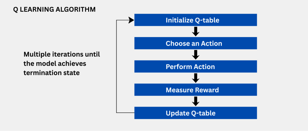
How Q-Learning Works: The Update Rule

The mechanical execution of Q-learning relies on an iterative mathematical update known as the Bellman equation, which continuously refines the expected value of actions. This dynamic process continuously balances the immediate environmental feedback received against the projected long-term benefits of subsequent states.

The standard Q-learning algorithm systematically stores its learned Q-values in a data structure known as a Q-table. Within a Q-table matrix, the rows represent all possible observable states, the columns represent all permissible actions, and the individual cell values hold the mathematically expected future rewards for those specific state-action pairs. Prior to training, this table is typically initialized to zero.

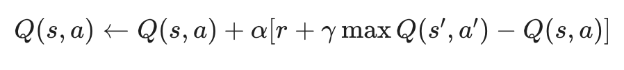
At each defined step, the algorithmic agent observes the current state, selects an action, and receives a scalar reward alongside the newly transitioned state. The agent subsequently updates the relevant Q-table matrix entry utilizing the Bellman equation update rule:

Hyperparameters and Exploration Strategies

Throughout the active training phase, the agent strategically manages the exploration-exploitation trade-off using an ε-greedy strategy. With probability ε, the agent executes a completely random action to aggressively explore the environment. Conversely, with probability 1-ε, the agent selects the action holding the highest known Q-value to actively exploit its current matrix knowledge. The mathematical parameter ε actively decays over the training timeline as the Q-values reliably converge. Given sufficient exploration iterations across all possible state-action pairs, Q-learning algorithms are mathematically guaranteed to converge to the optimal policy.

This temporal difference learning methodology relies on heavily tuned hyperparameters. The learning rate (a), typically defined within a range of 0.1 to 0.7, mathematically controls how rapidly new environmental information overwrites older value estimates. The discount factor (γ), constrained between 0 and 1, strictly dictates how much the computational agent values.

Q-Table vs. Function Approximation

While the tabular approach to Q-learning guarantees convergence in finite environments, it suffers from severe scalability limits when applied to complex, high-dimensional state spaces. Function approximation resolves this constraint by substituting the exhaustive Q-table with parameterized models like neural networks.

The primary engineering strength of a standard Q-table lies in its programmatic simplicity and distinct interpretability, alongside its absolute convergence guarantees within small, discrete environments. However, the Q-table data structure rapidly breaks down due to state space explosion. For instance, a basic 10×10 gridworld supporting 4 possible actions requires only 400 matrix entries. Conversely, rendering a modern video game environment yields a continuous state space that renders raw tabular storage entirely intractable.

To effectively scale the algorithm, engineers utilize function approximation. This technique replaces the discrete Q-table matrix with a parameterized mathematical function configured to approximate Q(s,a) continuously. A Deep Q-Network (DQN) operates as the canonical function approximator, utilizing a deep neural network specifically trained to accurately predict Q-values. The DQN architecture was famously utilized in DeepMind’s advanced Atari-playing agents.

To stabilize the volatile neural network training process, modern DQN frameworks introduce two critical architectural additions. An experience replay buffer is implemented to systematically break data sequence correlation, and an isolated target network is deployed to stabilize the continuous Bellman equation targets during backpropagation.

What are the Applications and Limitations of Q-Learning?

Beyond academic gridworld environments, Q-learning algorithms directly power distinct enterprise and industrial applications where optimal policy derivation is critical. However, software practitioners must meticulously account for inherent algorithmic limitations regarding sample efficiency and environment stationarity before progressing to production.

Enterprise use cases

Q-learning architectures excel strictly in environments that necessitate complex sequential decision-making. Prominent production use cases include deploying game-playing agents for advanced board games, managing automated robotic navigation telemetry, executing complex resource allocation, and maintaining dynamic network routing optimization. In specialized enterprise settings, Q-learning variants are heavily utilized for recommendation system policy optimization, executing adaptive process control loops, and driving the automation of dynamic A/B testing policies.

Operational constraints

Despite its vast utility, Q-learning possesses strict operational limitations. The fundamental limitation remains the computational inability of the basic Q-table matrix to scale, an architectural problem inherently addressed by migrating to robust DQN architectures. Furthermore, Q-learning mathematically struggles within sparse reward environments; if external feedback is highly infrequent, algorithmic convergence slows dramatically, often requiring advanced reward shaping engineering techniques to accurately mitigate.

Sample inefficiency serves as another major constraint. Basic Q-learning algorithms routinely require millions of discrete environment interactions to adequately learn an optimal policy, rendering it highly computationally expensive within real-world production settings. Finally, non-stationarity poses a persistent operational risk. If the underlying environment dynamics alter significantly after the agent is trained, the statically stored Q-values rapidly become outdated, necessitating rigorous periodic retraining protocols to maintain strict operational accuracy.

Q-Learning, Model Versioning, and the ML Pipeline

A converged Q-table or trained network is a machine learning artifact. Like any artifact in production, it needs governance: versioning, scanning, and reproducible deployment. Treating reinforcement learning outputs with the identical artifact management discipline applied to traditional software is absolutely essential for reproducible and auditable deployments.

Within modern software development workflows, a trained Q-learning agent must be explicitly treated as a definitive computational model artifact. Whether the generated artifact is a serialized Q-table matrix or a vast set of complex DQN neural network weights, it mathematically encodes the agent’s learned policy. It must be securely stored, strictly versioned, and maintained as entirely reproducible.

Experiment tracking and model registries

Integrating active Q-learning into an enterprise MLOps lifecycle fundamentally demands precise algorithmic experiment tracking. ML practitioners must systematically log all training hyperparameters, meticulously recording the learning rate, discount factor, and precise epsilon-decay operational schedules. Dedicated tracking tools capture comprehensive training episodes, scalar reward curves, and specific convergence metrics per execution run.

An enterprise ML Model registry must subsequently handle these specific RL agents, strictly versioning the serialized Q-tables alongside the explicit environment configurations utilized during the original training run. Maintaining exact artifact provenance and recording exactly which training datasets, environment framework versions, and hyperparameter sets produced each specific Q-table version ensures reliably auditable workflows. Serving a mature Q-learning agent in a live, real-time computational system requires the exact same latency optimization, dynamic scaling infrastructure, and rigorous monitoring discipline inherently applied to any standard production Model Registry deployment.

How JFrog Supports Reinforcement Learning Workflows

Q-learning fundamentally enables autonomous computational agents to rigorously derive optimal decision-making policies without requiring a pre-existing dynamic environmental model. Effectively integrating these heavily trained agents into enterprise production systems demands strict artifact governance and perfectly reproducible deployment pipelines to maintain high operational integrity.

As your organization aggressively scales its reinforcement learning initiatives, reliably managing the complex lifecycle of resulting Q-tables, DQN weights, and environment framework configurations introduces significant operational complexity and security risk. The JFrog Platform, featuring JFrog Artifactory and JFrog ML, provides a universal artifact repository and a highly comprehensive MLOps operational control layer that reliably secures and versions your RL artifacts. JFrog Artifactory acts as the universal artifact repository, strictly securing your Q-table binary files, configuration data, and essential training dependency packages with complete version history and auditable metadata lineage. Furthermore, JFrog Xray integrates seamlessly across the pipeline to actively surface known vulnerabilities within your Python packages and specialized ML frameworks prior to deployment.

Start a free trial or schedule a demo to see how JFrog supports reinforcement learning workflows.