Be Careful from Data Leakage – Potential Pitfalls in your Machine Learning Model
By Shon Mendelson, Data Scientist @JFrog
January 11, 2022
16 min read

Background
Consider the following scenario: you’ve worked months on a machine learning model with all the essential elements including feature engineering, feature selection, model selection, hyperparameters tuning, etc. Business approves and you deploy the model and suddenly, for the ongoing data, the results are not adding up. A common (and painful!) source of such difference in the results can be caused by data leakage. In the following article, I will explain what data leakage is, and what may cause data leakage to occur. I will also suggest a simple approach to tackle data leakage during the development stage.
Data Leakage & Technical Terms
Data leakage refers to a mistake that is made by the creator of a machine learning model in which information about the target variable is leaking into the input of the model during the training of the model; information that will not be available in the ongoing data that we would like to predict on.
Training set – a labeled data set that is used to train a model.
Validation set – a labeled data set that is used to evaluate the trained model.
Ongoing data (production) – unlabeled data that the trained model predicts on and creates predicted labels.
Data collection – the procedure of pulling the data from databases/source systems/etc.
Data preprocessing – the process of transforming raw data to make it applicable for our model. E.g., scaling the numeric features for optimization-based algorithms (neural network, SVM, logistic regression, etc.).
Data Leakage Challenges
Unlike over-fitting that we can detect by measuring the differences between the train-validation evaluation metric, data leakage is much more difficult to detect since both your train & validation can achieve great results but the results on the ongoing data will be drastically lower. Identifying the leakage once the model is already deployed in your production environment is not ideal. It would be much for us to identify it in the development stage.
How is Data Leaking?
Data leakage can reveal itself in many types of real-life scenarios. We will examine an example data set in relation to the source of the leaks that can be caused by: wrong data collection, wrong data processing, or biased sampling.
Consider the following dataset:
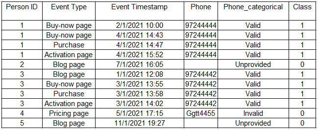
The table above is an example of transaction data. Every ID represents a person, and each row represents an action (visit on a company website page, purchase, etc.) on a specific timestamp. It also includes the phone number and a categorical variable that indicates whether it is valid, invalid, or unprovided. The class indicates whether the person purchased the product or not (binary variable).
To better understand it, let’s look at the first ID as an example: this person visited two times on the buy-now page (first two rows), purchased the product (third row), and visited once at the activation page (fourth row). He provided a valid phone number. Its class value is one since he purchased the product.
Let’s drill down to mistakes that may cause data leakage.
Wrong Data-collection
Data leakage can occur when we include information from future events. For example, we could count the number of visits on the activation page as an explanatory variable. But if we do so without time filtering we will teach the model: P(Purchase| number of visits in the activation page = 0) = 0.
Since we aim to predict whether a person will buy our product before the actual purchase this rule will not hold for the ongoing data, in which the persons didn’t buy the product yet, hence, might never visit the activation page though they have intent to purchase the product (at least some of them).
The more complicated scenario is when two events occur simultaneously. For example, we can see that each person that bought the product has visited the buy-now page a few minutes before the purchase. If we do not filter out these events, we again teach our model that each person that purchases the product visits the buy-now page. It might be true right before the purchase, but maybe a few hours before the purchase, the person has never visited the buy-now page though he already decided that he will purchase the product.
To avoid this kind of data leakage, we need to define each ID in the training data as its relevant date, to filter out events that occurred after it. The relevant date can be the date when an observation turned from class 0 to class 1 (the purchase date in our example), or, depending on the business needs, we can define how early we would like to predict the change in class and define the relevant date accordingly.
Another scenario of data leakage which arises from data collection is when a feature (or several features) is having dynamic updates that depend on the target variable. Following the above example, we can create a categorical feature from the phone number with three levels– unprovided, valid, and invalid. So far so good. However, if after the purchase the person is asked to provide a valid phone number, it makes it more complicated because the feature value might change due to the purchase. Our model will learn that P(Purchase| phone number invalid or not provided) = 0, which again isn’t true.
To avoid this kind of data leakage, make sure you understand exactly how each feature is collected and whether it’s going to be updated with relation to the class event.
Wrong Data-preprocessing
You created a query to produce the training data, and you aim to fit a supervised model. In most cases, some preprocessing is required. Preprocessing can be either unsupervised or supervised, and the latter is much more dangerous when it comes to data leakage.
An example of supervised preprocessing is target encoding. In target encoding, a categorical feature is encoded as the mean of the target variable. If it applied to all data without separation to train & validation, the encoded feature would seem to be better than it is since it contains information about the target variable, information that won’t be available in the ongoing data that does not have labels.
Unsupervised preprocessing (e.g., scaling) may not cause target leakage, but it can also cause an unreliable evaluation of your model if applied incorrectly.
The common approach is to compute the parameters of the preprocessing using the training data and apply it for both the training & ongoing data. I.e., use fit_transform() for the training data and transform() for the ongoing data. If you do so, do the same in the validation stage, i.e., split the data to training & validation, compute the parameters of the scaling (or any other preprocessing) on the training and then apply it for both the training & validation data.
To avoid this kind of data leakage/unreliable evaluation you can use scikit-learn pipelines.
Biased Sampling
In many real-life applications, labeled data is not well-organized. Following the above example – the positive class is well defined (those who purchased the product), and their relevant date is the purchase date.
For the non-purchase population, it’s a bit trickier. If your marketing team documents when they defined a person as unqualified (i.e., ~0 chance for purchase) – you can use it as the date they became class 0. But, otherwise, how will you know when exactly they didn’t buy the product (to filter out future events as discussed above)? Maybe they didn’t buy the product yet, but they are still in the process of evaluating the product?
If you choose today as the relevant date, you’ll get a biased population – the positive class is well spread in history whereas the negative class is focused on more recent data. The persons who purchased the product did it in different timestamps and the ones who did not purchase will all get relevant date = today. Instead of learning what distinguishes between persons who purchase the product and those who don’t purchase it, your model will learn how to distinguish between recent data and old data.
Data leakage appears not only in tabular data but also in NLP. Say you aim to build a classifier to distinguish between positive and negative sentiment (and say there are no public data sets exactly for that), so you ask one friend to write many positive-sentiment sentences and another friend to write many negative-sentiment sentences. The sentences might contain some information that does not relate to the fact that the sentence is positive or negative. For example, if the positive-sentiment writer tends to write shorter sentences than the negative-sentiment writer – you teach your model: P(positive| sentence is short) ~ 1, which is not necessarily true in the real-life ongoing data.
Data Leakage Will Destroy Your Machine Learning Model
I know I couldn’t choose a more dramatic title than this, but I truly believe that when your model includes leakage you cannot trust it for the ongoing data (at least not the same trust you had in the validation stage). The evaluation metrics will be more optimistic in the validation stage, but this is not the only problem. Additionally, the features that contain the leakage will be treated as much better in training than in the ongoing data; hence, our models will be built incorrectly because:
- The leaking features will get higher weights in the model than they should be (e.g., higher level of the tree for a decision-tree-based model).
- We will not be able to learn the real interactions of the leaking features with other features in the model.
- We might apply wrong feature engineering based on the leaking features.
Think about it, if you teach your model a direct relationship to the target variable (a relationship that does not observe in the ongoing data), such as the example above P(Purchase|phone number was not provided or invalid) = 0, you won’t let your model learn what affects the probability to purchase in case the phone number was not provided or invalid.
How to Detect Data Leakage?
If our goal was to detect the leakage in the ongoing predictions, we could monitor the difference between the distribution of the features (e.g., using KL divergence for a categorical feature). Though a change in a feature distribution does not necessarily point to data leakage, it can also be concept drift. But at least if we point out such a feature, we can validate the way we collect & process it.
We can also monitor the evaluation metrics and if there is a big difference it can point to data leakage (it can also be overfitting, but let’s assume that we make sure in the development stage that our model is not over-fitted).
These important concepts should also be applied for monitoring over time. In order to detect the leakage in the development stage, I’d suggest a simple, yet efficient, the method in a decision-tree-based model:
- Train a decision-tree-based model.
- Plot the feature importance.
- If you see a shape of a trunk, meaning the gap between the best feature to the second one is very (!) big. It means you can use only the first feature and achieve identical (or almost identical) results to those achieved by using all features. I am not saying there aren’t situations where a target variable may be predicted using only one or two features, but it isn’t the case for most real-life applications.
Keeping with the use-case above, let’s demonstrate this idea:
import pandas as pd
import numpy as np
from sklearn.ensemble import RandomForestClassifier
import matplotlib.pyplot as plt
import random
from datetime import timedelta
from sklearn.model_selection import train_test_split, cross_val_score
from sklearn.metrics import f1_score
First, I simulated transaction data as shown in the example above. For those who purchase the product, I simulated a visit on the activation page after the purchase.
Simulate Data
db_size = 10000
n_ids = 2500
df = pd.DataFrame()
df[‘ID’] = np.random.randint(n_ids, size=db_size)
events_types = [‘blog_page’, ‘product_page’, ‘pricing_page’, ‘purchase’]
df[‘event_type’] = random.choices(events_types, k=db_size,
                                  cum_weights=[0.5, 0.8, 0.98, 1])
df[‘event_timestamp’] = [pd.to_datetime(“today”)
                         - timedelta(hours=np.random.randint(24*30, size=1)[0].item())
                         for i in range(db_size)]
df.loc[df.event_type == ‘purchase’, ‘event_timestamp’] = df.loc[df.event_type == ‘purchase’, ‘event_timestamp’]
                                                                                               + timedelta(days=30)
Simulate Visits in the Activation-page after the Purchase
activations_df = pd.DataFrame(columns=df.columns)
i = 0
for ind in df[df.event_type == ‘purchase’].index:
    activations_df.loc[db_size + i] = [df.loc[ind, ‘ID’], ‘activation_page’,
                                       df.loc[ind, ‘event_timestamp’]
                                       + timedelta(minutes=np.random.randint(60, size=1)[0].item())]
    i += 1
df = pd.concat([df, activations_df], axis=0)
After that, I added positive labels for those who purchase the product. From those who didn’t purchase yet, I randomly chose some to be labeled as negative (say they are marked as unqualified by our marketing team). The rest do not have labels since they neither buy the product nor are marked as unqualified. They will be our ongoing data for this demonstration.
Add Labels
purchase_ids = df.loc[df.event_type == ‘purchase’, ‘ID’].unique()
none_purchase_ids_size = purchase_ids.shape[0] * 10
df[‘class’] = np.nan
df.loc[df[‘ID’].isin(purchase_ids), ‘class’] = 1
none_purchase_ids = random.sample(list(df.loc[df[‘class’].isnull(), ‘ID’].unique()), none_purchase_ids_size)
df.loc[df[‘ID’].isin(none_purchase_ids), ‘class’] = 0
Split to Training Data (with labels) and Ongoing Data (without labels)
df_train = df[~df[‘class’].isnull()]
df_test = df[df[‘class’].isnull()]
The following functions are used for the analysis. The first function is used to aggregate the transaction data – for each event type, I counted the number of times it appears as an explanatory variable. The second function is used to plot the feature importance.
Useful Functions
Feature Aggregation
def aggregate_data(data, is_train=True):
    by = [‘ID’, ‘class’] if is_train else [‘ID’]
    data = data.groupby(by=by, as_index=False).agg(
                count_blog=(‘event_type’, lambda x: np.sum(x == ‘blog_page’)),
                count_product=(‘event_type’, lambda x: np.sum(x == ‘product_page’)),
                count_pricing=(‘event_type’, lambda x: np.sum(x == ‘pricing_page’)),
                count_activation=(‘event_type’, lambda x: np.sum(x == ‘activation_page’)))
    return data
Plot Feature Importance
def plot_feature_importance(X_train, model):
    features = X_train.columns
    importances = model.feature_importances_
    indices = np.argsort(importances)
    plt.title(‘Feature Importance’)
    plt.barh(range(len(indices)), importances[indices], color=‘b’, align=‘center’)
    plt.yticks(range(len(indices)), [features[i] for i in indices])
    plt.xlabel(‘Relative Importance’)
    plt.show()
Here I used the function above to aggregate the ongoing data.
Aggregate the Ongoing Data
df_test = aggregate_data(df_test, is_train=False)
X_ongoing = df_test.drop([‘ID’], axis=1)
Here is an example of data leakage. I didn’t filter out future events.
Data Leakage (including future events)
df_train_leakage = df_train[df_train.event_type != ‘purchase’]
df_train_leakage = aggregate_data(df_train_leakage)
X, y = df_train_leakage.drop([‘ID’, ‘class’], axis=1), df_train_leakage[‘class’]
rf = RandomForestClassifier(class_weight=‘balanced’)
Evaluation
X_train, X_test, y_train, y_test = train_test_split(X, y, test_size=0.2, stratify=y)
rf.fit(X_train, y_train)
y_pred = rf.predict(X_test)
score = f1_score(y_true=y_test, y_pred=y_pred)
print(‘The F1 score is: ’ + str(np.round(score, 2)))
The F1 score is 1.0My evaluation is perfect. But it is not because I developed an awesome model. It is because I had data leakage that led my model to learn P(Purchase| visit in the activation page) = 1.
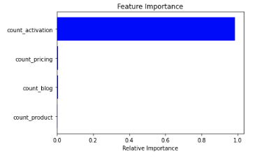
The feature importance plot also suggests the count_activation feature is very good. “Too good to be true”.
Predictions for the Ongoing Data
y_pred_leakage = rf.predict(X_ongoing)
positive_frac_predicted = y_pred_leakage.mean()
print(‘The predictions for ’ + str(np.round(positive_frac_predicted, 2) * 100) + ‘% of the persons is positive (purchase)’)
The predictions for 0% of the persons is positive (purchase)We can also see that even though our evaluation was perfect, our model predicted that no one in the ongoing data will purchase our product. Pretty sad.
Here I started with excluding future events.
Without Data Leakage (excluding future events)
purchase_dates = df_train.loc[df_train.event_type == ‘purchase’, [‘ID’, ‘event_timestamp’]]
purchase_dates.columns = [‘ID’, ‘purchase_timestamp’]
df_train_no_leakage = df_train.merge(purchase_dates, how=‘left’)
df_train_no_leakage = df_train_no_leakage[(df_train_no_leakage.event_timestamp <
                                           df_train_no_leakage.purchase_timestamp)
                                          | (df_train_no_leakage.purchase_timestamp.isnull())]
df_train_no_leakage = aggregate_data(df_train_no_leakage)
X, y = df_train_no_leakage.drop([‘ID’, ‘class’], axis=1), df_train_no_leakage[‘class’]
rf = RandomForestClassifier(class_weight=‘balanced’)
Evaluation
X_train, X_test, y_train, y_test = train_test_split(X, y, test_size=0.2, stratify=y)
rf.fit(X_train, y_train)
y_pred = rf.predict(X_test)
score = f1_score(y_true=y_test, y_pred=y_pred)
print(‘The F1 score is: ’ + str(np.round(score, 2)))
The F1 score is: 0.07We can see the evaluation is much lower.
plot_feature_importance(X_train=X_train, model=rf)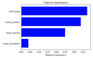
The feature importance looks normal.
Predictions for the Ongoing Data
y_pred_no_leakage = rf.predict(X_ongoing)
positive_frac_predicted = y_pred_no_leakage.mean()
print(‘The predictions for ’ + str(np.round(positive_frac_predicted, 2) * 100) + ‘% of the persons is positive (purchase)’)
The predictions for 26% of the persons is positive (purchase)For the ongoing data, some predicted as a potential to purchase our product.
Extension – Data Leakage in Computer-vision
In computer vision, irrelevant information can leakage into the images that can make the neural network learn a rule that will be awesome in the development stage but useless for the ongoing data.
Say you aim to distinguish between healthy and infected plants by a single image. For that, you design an experiment to get some labeled data. Skip the biological aspect of it – say you need to apply some process to make some of the plant infected (the positive class) and say this process takes more than one day. How would you remember which plants are part of the ongoing process to become infected and which are not? The simplest solution is to mark them. Group A – infected plants and group B – healthy plants. You are ending up with images and labels. The only problem is that the images contain information about the target variable – the positive class marked with “A” and the negative class marked with “B”.
If you train a deep-neural network directly on the images it will learn to identify the letter “A” or “B” to classify whether a plant is infected or healthy. In the real world, the plants won’t be marked, hence, the model that learned the label from the image will collapse for the ongoing data.
Another similar example is that the different classes are pictured at different times in the day. Hence, instead of learning what characterized an infected plant, you learn how to distinguish between day and night.
Final Words
Hopefully, you can now see how common a phenomenon of data leakage is, and how every data scientist should be familiar with it. While being careful and cautious is important, It is important to remember that not every shift in an evaluation metric or feature distribution is a direct cause of data leakage. Yet, by understanding the relationship between the features to the target variable, and knowing exactly how your features are collected, you will still be able to keep an eye for data leakage that can cause harm to your model.